43 format data labels excel 2016
Format Data Labels Vertically using Pareto in Excel 2016 Re: Format Data Labels Vertically using Pareto in Excel 2016. Try this: Right-click on one of the data labels > Format Data Labels > Size & Properties > Alignment > Text direction: Stacked. Register To Reply. 10-03-2017, 01:19 PM #3. 1gambit. View Profile. How to Print Labels from Excel - Lifewire Choose Start Mail Merge > Labels . Choose the brand in the Label Vendors box and then choose the product number, which is listed on the label package. You can also select New Label if you want to enter custom label dimensions. Click OK when you are ready to proceed. Connect the Worksheet to the Labels
Format Data Labels in Excel- Instructions - TeachUcomp, Inc. To do this, click the "Format" tab within the "Chart Tools" contextual tab in the Ribbon. Then select the data labels to format from the "Chart Elements" drop-down in the "Current Selection" button group. Then click the "Format Selection" button that appears below the drop-down menu in the same area.

Format data labels excel 2016
Change Horizontal Axis Values in Excel 2016 - AbsentData 1. Select the Chart that you have created and navigate to the Axis you want to change. 2. Right-click the axis you want to change and navigate to Select Data and the Select Data Source window will pop up, click Edit 3. The Edit Series window will open up, then you can select a series of data that you would like to change. 4. Click Ok Edit titles or data labels in a chart - support.microsoft.com The first click selects the data labels for the whole data series, and the second click selects the individual data label. Right-click the data label, and then click Format Data Label or Format Data Labels. Click Label Options if it's not selected, and then select the Reset Label Text check box. Top of Page How to add or move data labels in Excel chart? To add or move data labels in a chart, you can do as below steps: In Excel 2013 or 2016. 1. Click the chart to show the Chart Elements button . 2. Then click the Chart Elements, and check Data Labels, then you can click the arrow to choose an option about the data labels in the sub menu. See screenshot: In Excel 2010 or 2007
Format data labels excel 2016. How to hide zero data labels in chart in Excel? If you want to hide zero data labels in chart, please do as follow: 1. Right click at one of the data labels, and select Format Data Labels from the context menu. See screenshot: 2. In the Format Data Labels dialog, Click Number in left pane, then select Custom from the Category list box, and type #"" into the Format Code text box, and click Add button to add it to Type list box. How to format axis labels as thousands/millions in Excel? 1. Right click at the axis you want to format its labels as thousands/millions, select Format Axis in the context menu. 2. In the Format Axis dialog/pane, click Number tab, then in the Category list box, select Custom, and type [>999999] #,,"M";#,"K" into Format Code text box, and click Add button to add it to Type list. See screenshot: 3. support.microsoft.com › en-us › officeTutorial: Import Data into Excel, and Create a Data Model With the data still highlighted, press Ctrl + T to format the data as a table. You can also format the data as a table from the ribbon by selecting HOME > Format as Table. Since the data has headers, select My table has headers in the Create Table window that appears, as shown here. Formatting the data as a table has many advantages. How to Customize Your Excel Pivot Chart Data Labels - dummies To remove the labels, select the None command. If you want to specify what Excel should use for the data label, choose the More Data Labels Options command from the Data Labels menu. Excel displays the Format Data Labels pane. Check the box that corresponds to the bit of pivot table or Excel table information that you want to use as the label.
Creating a chart with dynamic labels - Microsoft Excel 2016 1. Right-click on the chart and in the popup menu, select Add Data Labels and again Add Data Labels : 2. Do one of the following: For all labels: on the Format Data Labels pane, in the Label Options, in the Label Contains group, check Value From Cells and then choose cells: For the specific label: double-click on the label value, in the popup ... Excel 2016: How to Format Data and Cells - UniversalClass.com To do this, go to the Format Cells dialogue box again, and click Custom n the category column. In the Type list, select the format that you want to customize. As you can see in the snapshot above, we chose the currency format. Now go to the Type field and customize the format by entering the format you want to use. Click OK when you're finished. peltiertech.com › cusCustom Axis Labels and Gridlines in an Excel Chart Jul 23, 2013 · Select the vertical dummy series and add data labels, as follows. In Excel 2007-2010, go to the Chart Tools > Layout tab > Data Labels > More Data label Options. In Excel 2013, click the “+” icon to the top right of the chart, click the right arrow next to Data Labels, and choose More Options…. Change the format of data labels in a chart To get there, after adding your data labels, select the data label to format, and then click Chart Elements > Data Labels > More Options. To go to the appropriate area, click one of the four icons ( Fill & Line, Effects, Size & Properties ( Layout & Properties in Outlook or Word), or Label Options) shown here.
Excel 2016 Tutorial Formatting Data Labels Microsoft ... FREE Course! Click: about Formatting Data Labels in Microsoft Excel at . A clip from Mastering Excel M... 3D maps excel 2016 add data labels Re: 3D maps excel 2016 add data labels. I don't think there are data labels equivalent to that in a standard chart. The bars do have a detailed tool tip but that required the map to be interactive and not a snapped picture. You could add annotation to each point. Select a stack and right click to Add annotation. Cheers. Format Data Label: Label Position - Microsoft Community when you add labels with the + button next to the chart, you can set the label position. In a stacked column chart the options look like this: For a clustered column chart, there is an additional option for "Outside End" When you select the labels and open the formatting pane, the label position is in the series format section. Does that help? Excel 2010: How to format ALL data point labels ... There's no option to for example, right click and select "all data point labels." Now if I just select the whole graph and then change the font size, it changes everything (of course) title, axes labels, etc. I'd like to just increase the size of all data point labels on the graph.

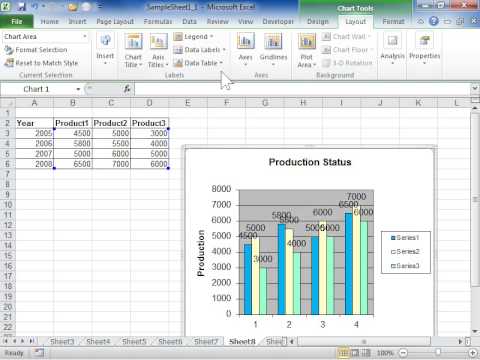
Chapter 3 Excel 2007/2010 Charts
Adding Data Labels to Your Chart (Microsoft Excel) To add data labels in Excel 2013 or Excel 2016, follow these steps: Activate the chart by clicking on it, if necessary. Make sure the Design tab of the ribbon is displayed. (This will appear when the chart is selected.) Click the Add Chart Element drop-down list. Select the Data Labels tool.
Print column headers or spreadsheet labels on every page - Microsoft Excel 2016
stackoverflow.com › questions › 48559387stacked column chart for two data sets - Excel - Stack Overflow Feb 01, 2018 · I wonder if there is some way (also using VBA, if needed) to create a stacked column chart displaying two different data sets in MS Excel 2016. Looking around, I saw the same question received a positive answer when working with Google Charts (here's the thread stacked column chart for two data sets - Google Charts)
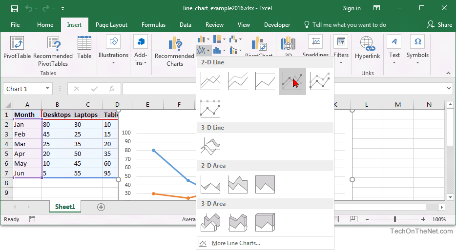
MS Excel 2016: How to Create a Line Chart
How to Create Mailing Labels in Excel | Excelchat Step 1 - Prepare Address list for making labels in Excel First, we will enter the headings for our list in the manner as seen below. First Name Last Name Street Address City State ZIP Code Figure 2 - Headers for mail merge Tip: Rather than create a single name column, split into small pieces for title, first name, middle name, last name.
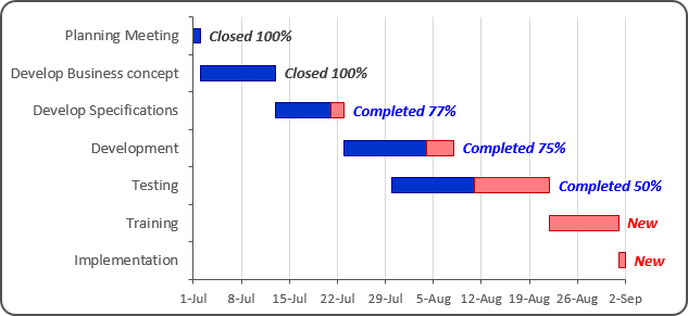
Gantt chart with progress - Microsoft Excel undefined
How to create Custom Data Labels in Excel Charts Right click on any data label and choose the callout shape from Change Data Label Shapes option. Now adjust each data label as required to avoid overlap. Put solid fill color in the labels Finally, click on the chart (to deselect the currently selected label) and then click on a data label again (to select all data labels).

Repeat item labels in a PivotTable
support.microsoft.com › en-us › officeAdd or remove data labels in a chart - support.microsoft.com Right-click the data series or data label to display more data for, and then click Format Data Labels. Click Label Options and under Label Contains , select the Values From Cells checkbox. When the Data Label Range dialog box appears, go back to the spreadsheet and select the range for which you want the cell values to display as data labels.

Excel Treemap - Beat Excel!
› excel_2016 › tipsCreating a simple thermometer chart - Microsoft Excel 2016 Choose the Clustered Column chart.. 3. Remove the horizontal (x) axis.. 4. In the thermometer chart, the column width is equal to the chart width. To make the column occupy the entire width of the plot area, double-click the column to display the Format Data Point task pane (or choose it in the popup menu).
Excel 2010 Remove Data Labels from a Chart - YouTube
Excel Charts: Creating Custom Data Labels - YouTube In this video I'll show you how to add data labels to a chart in Excel and then change the range that the data labels are linked to. This video covers both W...

Excel 3-D Pie Charts
Move data labels - support.microsoft.com Click any data label once to select all of them, or double-click a specific data label you want to move. Right-click the selection > Chart Elements > Data Labels arrow, and select the placement option you want. Different options are available for different chart types.

How to Add Data Labels in Excel - Excelchat | Excelchat
excel - Change format of all data labels of a single ... Change the format of labels. Remove added contents. Workaround 2: Change to a dummy range for the data labels, which has no empty cells. Change the format of labels. Switch back to your intended range. This might require The XY Chart Labeler, an excellent add-in by Rob Bovey.
Post a Comment for "43 format data labels excel 2016"