39 excel pivot table 2 row labels

Pivot Table "Row Labels" Header Frustration - Microsoft Tech Community Enabling Remote Work. Small and Medium Business. Humans of IT. Empowering technologists to achieve more by humanizing tech. Green Tech. Raise awareness about sustainability in the tech sector. MVP Award Program. Find out more about the Microsoft MVP Award Program. How to Customize Your Excel Pivot Chart Data Labels - dummies The Data Labels command on the Design tab's Add Chart Element menu in Excel allows you to label data markers with values from your pivot table. When you click the command button, Excel displays a menu with commands corresponding to locations for the data labels: None, Center, Left, Right, Above, and Below. None signifies that no data labels ...

Pivot Table Sort by second row label - Microsoft Community EXCEL 2010 Windows 7. I have a very simple pivot table with two row labels - number and name. the "values" are points. Column A is number, column B has name, and column C has the sum of points. How can I sort the pivot table by column B (Name)? This thread is locked. You can follow the question or vote as helpful, but you cannot reply to this ...

Excel pivot table 2 row labels

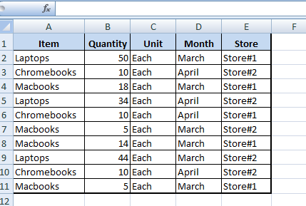
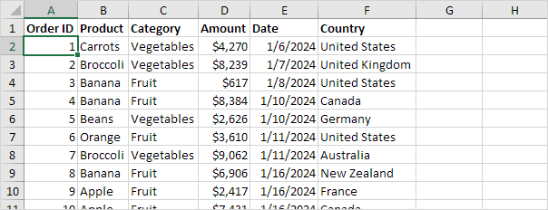
Pivot Table adding "2" to value in answer set 1) Right click your pivot table -> Pivot table options -> Data -> Change "Number of items to retain per field" to NONE. 2) Wipe all rows in your data source except for the headers. 3) Refresh the pivot table. 4) Save, and close all instances of Excel. 5) Reopen the file, and paste your data. 6) Refresh the pivot table. How to repeat row labels for group in pivot table? - ExtendOffice 1. Firstly, you need to expand the row labels as outline form as above steps shows, and click one row label which you want to repeat in your pivot table. 2. Then right click and choose Field Settings from the context menu, see screenshot: 3. In the Field Settings dialog box, click Layout & Print tab, then check Repeat item labels, see screenshot: Multi-level Pivot Table in Excel (In Easy Steps) First, insert a pivot table. Next, drag the following fields to the different areas. 1. Country field to the Rows area. 2. Amount field to the Values area (2x). Note: if you drag the Amount field to the Values area for the second time, Excel also populates the Columns area. Pivot table: 3. Next, click any cell inside the Sum of Amount2 column. 4.

Excel pivot table 2 row labels. Sum of two column labels in pivot table - excelforum.com Re: Sum of two column labels in pivot table. Use Slicer. (usuall Ctrl+click or Shift+click combination for multiple items) Attached Files. PT.xlsx‎ (17.1 KB, 6 views) Download. How to rename group or row labels in Excel PivotTable? To rename Row Labels, you need to go to the Active Field textbox. 1. Click at the PivotTable, then click Analyze tab and go to the Active Field textbox. 2. Now in the Active Field textbox, the active field name is displayed, you can change it in the textbox. You can change other Row Labels name by clicking the relative fields in the PivotTable ... Pivot table - Wikipedia Row labels are used to apply a filter to one or more rows that have to be shown in the pivot table. For instance, if the "Salesperson" field is dragged on this area then the other output table constructed will have values from the column "Salesperson", i.e. , one will have a number of rows equal to the number of "Sales Person". How to make row labels on same line in pivot table? Make row labels on same line with PivotTable Options. You can also go to the PivotTable Options dialog box to set an option to finish this operation.. 1.Click any one cell in the pivot table, and right click to choose PivotTable Options, see screenshot:. 2.

Repeat item labels in a PivotTable - support.microsoft.com Right-click the row or column label you want to repeat, and click Field Settings. Click the Layout & Print tab, and check the Repeat item labels box. Make sure Show item labels in tabular form is selected. When you edit any of the repeated labels, the changes you make are applied to all other cells with the same label. Pivot Tables - Two Dimensions in Row Labels | MrExcel Message Board I'm trying to put two dimensions in my row labels - Organizations and Accounts. The... Forums. New posts Search forums. ... Excel Questions . Pivot Tables - Two Dimensions in Row Labels ... . Pivot Tables - Two Dimensions in Row Labels. Thread starter shanson; Start date May 8, 2012 ... Pivot table row labels side by side - Excel Tutorials E01. Paint damage. 3. Now, let's create a pivot table ( Insert >> Tables >> Pivot Table) and check all the values in Pivot Table Fields. Fields should look like this. Right-click inside a pivot table and choose PivotTable Options…. Check data as shown on the image below. The table is going to change. The pivot table is almost ready. How to make row labels on same line in pivot table? 1. Click any cell in your pivot table, and the PivotTable Tools tab will be displayed. 2. Under the PivotTable Tools tab, click Design > Report Layout > Show in Tabular Form, see screenshot: 3. And now, the row labels in the pivot table have been placed side by side at once, see screenshot:

Multiple row labels on one row in Pivot table | MrExcel Message Board In Excel 2003, a pivot table would allow you to place multiple row labels on the left hand side of a pivot table. I can't figure out how to make that happen in Excel 2010. I need material and material description on the lefthand side of the pivot table but it is placing the description underneath on a 2nd row form the material number. Design the layout and format of a PivotTable Click anywhere in the PivotTable. This displays the PivotTable Tools tab on the ribbon. On the Options tab, in the PivotTable group, click Options. In the PivotTable Options dialog box, click the Layout & Format tab, and then under Layout, select or clear the Merge and center cells with labels check box. Pivot Table Row Labels | MrExcel Message Board 3,699. May 20, 2011. #6. rorya said: In 2010 you can do this. Right-click the row field, choose Field Settings, then on the Layout and Print tab, check the 'Repeat item labels' option. Click to expand... Rorya, Thanks, this resource of Excel 2010 I didn't know. Values appear twice in PivotTable row labels [SOLVED] The numbers are listed twice because they appear both as numbers and as text in your data. To change them all to numbers, type 0 into a cell, copy this then Paste Special - Values - Add. Then refresh the pivot table and it will display the numbers once. Register To Reply. 01-31-2010, 08:20 PM #3.

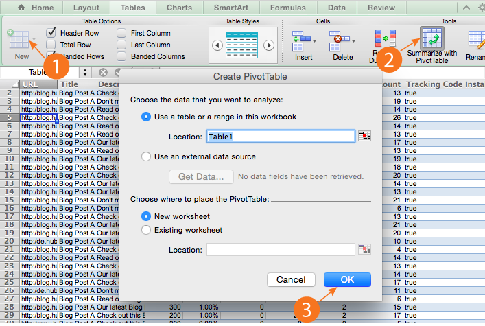
How to Create a Pivot Table in Excel: A Step-by-Step Tutorial (With Video)

Pivot Table Row Labels In the Same Line - Beat Excel! It is a common issue for users to place multiple pivot table row labels in the same line. You may need to summarize data in multiple levels of detail while rows labels are side by side. In this post I'm going to show you how to do it. ... After creating a pivot table in Excel, you will see the row labels are listed in only one column. But, if ...

Excel Pivot Table Report - Sort Data in Row & Column Labels & in Values Area, use Custom Lists

Filtering Grand Total Amounts Within Excel Pivot Tables Figure 3: The pivot table allows you to filter for specific columns. You can filter rows in a similar fashion, as shown in Figure 4: Click the arrow in the Row Labels field. Type the word Fruit in the Search Box (or manually filter in Excel 2007 and earlier). Click OK. The pivot table now only has rows for vendors that have the word Fruit in ...

Sorting a numeric field in my Pivot Table is greyed out. : excel

Duplicate Items Appear in Pivot Table - Excel Pivot Tables In Row 2 of the new column, enter the formula =TRIM(C2). Copy the formula down to the last row of data in the source table. If the source data is stored in an Excel Table, the formula should copy down automatically. Refresh the pivot table ; Remove the City field from the pivot table, and add the CityName field to replace it. _____

How to Create Pivot Table in Excel

get a row label from pivot table - Microsoft Tech Community Alternatively you may work with cube assuming you are at least on Excel 2010, as I remember it's the first which supports data model. Create PivotTable and after that convert it to cube formulas. Now you may take these formulas and convert it to form you need, for example. =CUBEVALUE( "ThisWorkbookDataModel", CUBEMEMBER("ThisWorkbookDataModel ...

Excel Pivot Table Report - Sort Data in Row & Column Labels & in Values Area, use Custom Lists

Pivot table row labels in separate columns • AuditExcel.co.za The issue here is simply that the more recent versions of Excel use this as the default report format. Our preference is rather that the pivot tables are shown in tabular form (all columns separated and next to each other). You can do this by changing the report format. So when you click in the Pivot Table and click on the DESIGN tab one of the ...

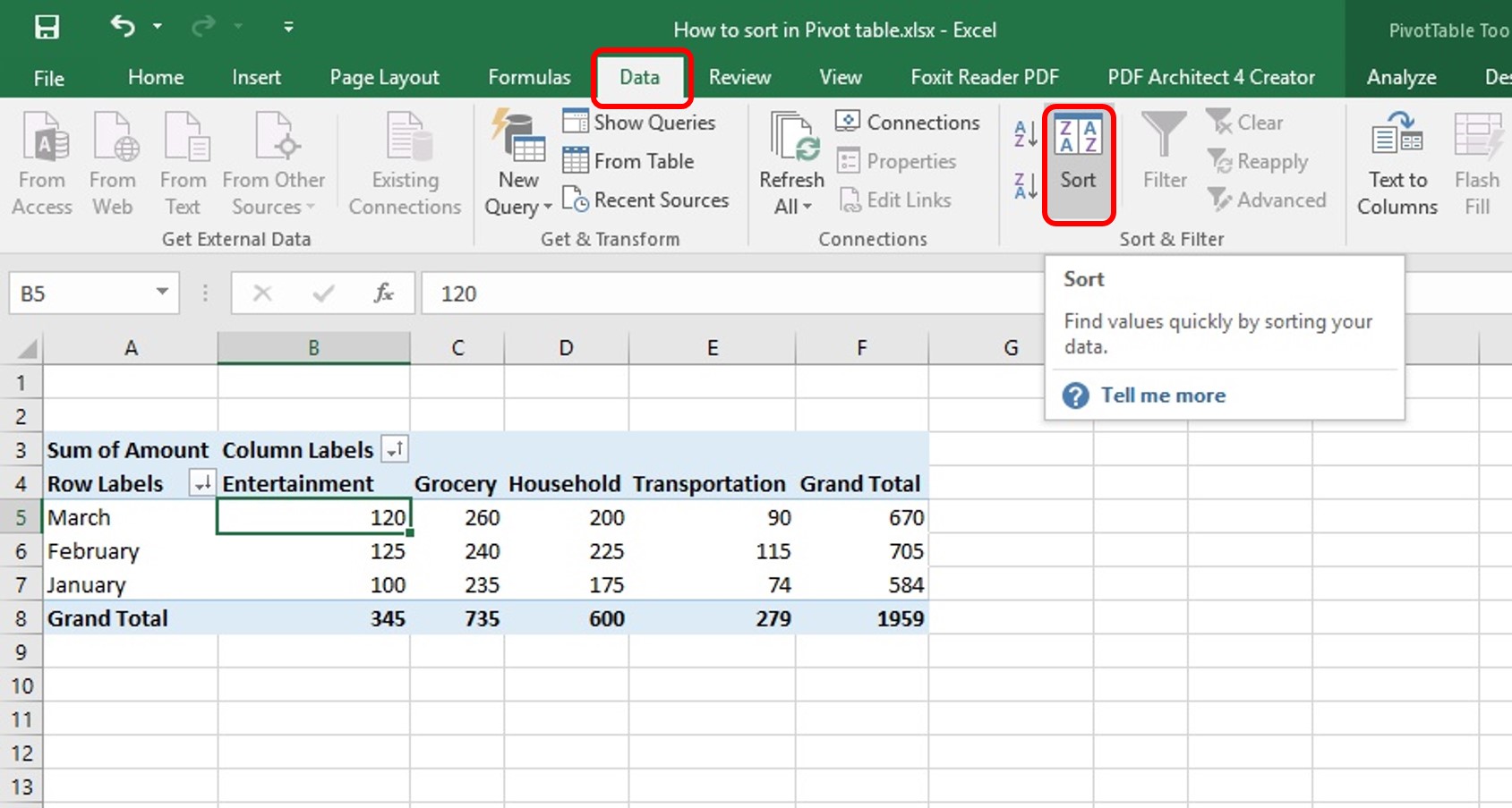
How to Sort Pivot Table | Custom Sort Pivot Table | A-Z, Z-A Order

Automatic Row And Column Pivot Table Labels - How To Excel At Excel Select the Insert Tab. Hit Pivot Table icon. Next select Pivot Table option. Select a table or range option. Select to put your Table on a New Worksheet or on the current one, for this tutorial select the first option. Click Ok. The Options and Design Tab will appear under the Pivot Table Tool. Select the check boxes next to the fields you want ...

Creating Pivot Tables in Excel for Exported Data – Teaching & Learning

Multi-level Pivot Table in Excel (In Easy Steps) First, insert a pivot table. Next, drag the following fields to the different areas. 1. Country field to the Rows area. 2. Amount field to the Values area (2x). Note: if you drag the Amount field to the Values area for the second time, Excel also populates the Columns area. Pivot table: 3. Next, click any cell inside the Sum of Amount2 column. 4.

Frequency Distribution in Excel - Easy Excel Tutorial

How to repeat row labels for group in pivot table? - ExtendOffice 1. Firstly, you need to expand the row labels as outline form as above steps shows, and click one row label which you want to repeat in your pivot table. 2. Then right click and choose Field Settings from the context menu, see screenshot: 3. In the Field Settings dialog box, click Layout & Print tab, then check Repeat item labels, see screenshot:

Share :